Technical Documentation

The downscaling workflow predicts carbon pools (Soil Organic Carbon and Aboveground Biomass) for cropland fields in California and then aggregates these predictions to the county scale.

It uses an ensemble-based approach to uncertainty propagation and analysis, maintaining ensemble structure to propagate errors through the prediction and aggregation processes.

Spatial downscaling workflow using machine learning with environmental covariates

Terminology

• Design Points: Fields chosen via stratified random sampling using k-means clustering on environmental data layers across California crop fields.
• Crop Fields: All croplands in the LandIQ dataset.
• Anchor Sites: Sites used as ground truth for calibration and validation, including UC research stations and Ameriflux sites.

This Repository Contains Two Workflows That Will Be Split

TODO Workflows (1 & 3) are in this repository and will be split

The workflows are

1. Site Selection: uses environmental variables (later also management layers) to create clusters and then select representative sites. The design_points.csv are then passed to the ensemble workflow
   
2. Ensemble in ccmmf/workflows repository, generates ensemble outputs
3. Downscaling: uses ensemble outputs to make predictions for each field in CA then aggregate to county level summaries.

Workflow Steps

Configuration

Workflow settings are configured in 000-config.R.

The configuration script reads the CCMMF directory from the environment variable CCMMF_DIR (set in .Renviron), and uses it to define paths for inputs and outputs.

The CCMMF_DIR variable, however, is defined in .Renviron so that it can: - Be used to locate and override R library (RENV_PATHS_LIBRARY) and cache (RENV_PATHS_CACHE) paths outside the home directory. - Be easily overridden via a shell export (export CCMMF_DIR=…) without modifying workflow scripts.

Configuration setup

To set up this workflow to run on your system, follow the following steps.

Clone Repository

git clone git@github.com:ccmmf/downscaling

• CCMMF_DIR should point to the shared CCMMF directory. This is the location where data, inputs, and outputs will be stored, as well as the location of the renv cache and library
• RENV_PATHS_CACHE and RENV_PATHS_LIBRARY store the renv cache and library in the CCMMF directory. These are in a subdirectory of the CCMMF directory in order to make them available across all users (and because on some computers, they exceed allocated space in the home directory).
• R_LIBS_USER must point to the platform and R version specific subdirectory inside RENV_PATHS_LIBRARY.
  
• .Rprofile
  • sets repositories from which R packages are installed
  • runs renv/activate.R
• 000-config.R
  • set pecan_outdir based on the CCMMF_DIR.
  • confirm that relative paths (data_raw, data, cache) are correct.
  • detect and use resources for parallel processing (with future package); default is available cores - 1
  • PRODUCTION mode setting. For testing, set PRODUCTION to FALSE. This is much faster and requires fewer computing resources because it subsets large datasets. Once a test run is successful, set PRODUCTION to TRUE to run the full workflow.

Management Scenario Configuration

To compare carbon outcomes under different agricultural practices, enable management scenario mode:

USE_PHASE_3_SCENARIOS <- TRUE

When enabled, the workflow processes multiple management scenarios in a single run. Each scenario represents a different combination of practices applied to annual croplands.

Available Management Scenarios:

Scenario	Description
baseline	Conventional management practices
compost	Compost application replacing mineral N fertilizer
reduced_till	Reduced tillage intensity (0.10)
zero_till	No tillage (0.00)
reduced_irrig_drip	Drip irrigation replacing canopy irrigation
stacked	Combined: compost + reduced tillage + drip irrigation

1. Data Preparation

Rscript scripts/009_update_landiq.R
Rscript scripts/010_prepare_covariates.R
Rscript scripts/011_prepare_anchor_sites.R

These scripts prepare data for clustering and downscaling:

• Converts LandIQ-derived shapefiles to a geopackage with geospatial information and a CSV with other attributes
• Extracts environmental covariates (clay, organic carbon, topographic wetness, temperature, precipitation, solar radiation, vapor pressure)
• Groups fields into Cal-Adapt climate regions
• Assigns anchor sites to fields

Inputs:

• LandIQ Crop Map: data_raw/i15_Crop_Mapping_2016_SHP/i15_Crop_Mapping_2016.shp
• Soilgrids: clay_0-5cm_mean.tif and ocd_0-5cm_mean.tif Consider aggregating 0-5,5-15,15-30 into a single 0-30 cm layer
• TWI: TWI/TWI_resample.tiff
• ERA5 Met Data: Files in GridMET/ folder named ERA5_met_<YYYY>.tiff
• Anchor Sites: data_raw/anchor_sites.csv

Outputs:

• ca_fields.gpkg: Spatial information from LandIQ
• ca_field_attributes.csv: Site attributes including crop type
• site_covariates.csv: Environmental covariates for each field
• anchor_sites_ids.csv: Anchor site information

Environmental Covariates

Variable	Description	Source	Units
temp	Mean annual temperature	ERA5	°C
precip	Mean annual precipitation	ERA5	mm/year
srad	Solar radiation	ERA5	W/m²
vapr	Vapor pressure deficit	ERA5	kPa
clay	Clay content	SoilGrids	%
ocd	Organic carbon density	SoilGrids	g/kg
twi	Topographic wetness index	SRTM-derived	-

2. Design Point Selection

Rscript scripts/020_cluster_and_select_design_points.R
Rscript scripts/021_clustering_diagnostics.R

Uses k-means clustering to select representative fields plus anchor sites:

• Subsample LandIQ fields and include anchor sites for clustering
• Select cluster number based on the Elbow Method
• Cluster fields using k-means based on environmental covariates
• Select design points from clusters for SIPNET simulation

Inputs: - data/site_covariates.csv - data/anchor_sites_ids.csv

Output: - data/design_points.csv

3. SIPNET Model Runs

A separate workflow prepares inputs and runs SIPNET simulations for the design points.

Inputs: - design_points.csv - Initial conditions (from modeling workflow)

Outputs: - out/ENS-<ensemble_number>-<site_id>/YYYY.nc: NetCDF files containing SIPNET outputs, in PEcAn standard model output format. - out/ENS-<ensemble_number>-<site_id>/YYYY.nc.var: List of variables included in SIPNET output (see table below)

Available Variables

Each output file named YYYY.nc has an associated file named YYYY.nc.var. This file contains a list of variables included in the output. SIPNET outputs have been converted to PEcAn standard units and stored in PEcAn standard NetCDF files. PEcAn standard units are SI, following the Climate Forecasting standards:

• Mass pools: kg / m2
  • TotSoilCarb: Total Soil Carbon
  • AbvGrndWood: Above ground woody biomass
• Mass fluxes: kg / m2 / s-1
  • GPP: Gross Primary Productivity
  • NPP: Net Primary Productivity
• Energy fluxes: W / m2
• Other:
  • LAI: m2 / m2

Variable	Description
GPP	Gross Primary Productivity
NPP	Net Primary Productivity
TotalResp	Total Respiration
AutoResp	Autotrophic Respiration
HeteroResp	Heterotrophic Respiration
SoilResp	Soil Respiration
NEE	Net Ecosystem Exchange
AbvGrndWood	Above ground woody biomass
leaf_carbon_content	Leaf Carbon Content
TotLivBiom	Total living biomass
TotSoilCarb	Total Soil Carbon
Qle	Latent heat
Transp	Total transpiration
SoilMoist	Average Layer Soil Moisture
SoilMoistFrac	Average Layer Fraction of Saturation
SWE	Snow Water Equivalent
litter_carbon_content	Litter Carbon Content
litter_mass_content_of_water	Average layer litter moisture
LAI	Leaf Area Index
fine_root_carbon_content	Fine Root Carbon Content
coarse_root_carbon_content	Coarse Root Carbon Content
GWBI	Gross Woody Biomass Increment
AGB	Total aboveground biomass
time_bounds	history time interval endpoints

4. Extract SIPNET Output

First, uncompress the model output. Only the netCDF files are needed.

# Set paths
ccmmf_dir=/projectnb2/dietzelab/ccmmf
archive_file="$ccmmf_dir/lebauer_agu_2025_20251210.tgz"
output_dir="$ccmmf_dir/modelout/ccmmf_phase_3_scenarios_20251210"

# Ensure output directory exists
mkdir -p "$output_dir"

# 
tar --use-compress-program="pigz -d" -xf \
  "$archive_file" \
  -C "$output_dir" \
  --strip-components=1 \
  --no-same-owner #\
#  --wildcards \
#  'lebauer_agu_2025/output_/out/' \
#  'lebauer_agu_2025/output_/out/ENS--/[0-9][0-9][0-9][0-9].nc'

Rscript scripts/030_extract_sipnet_output.R

Extracts and formats SIPNET outputs for downscaling:

• Extract output variables (AGB, TotSoilCarb) from SIPNET simulations
• Aggregate site-level ensemble outputs into long and 4D array formats
• Save CSV and NetCDF files following EFI standards

Inputs: - out/ENS-<ensemble_number>-<site_id>/YYYY.nc - results_monthly_<variable>.Rdata (management scenario mode) - site_info.csv (management scenario mode)

Outputs: - out/ensemble_output.csv: Long format data with columns: - scenario: Management scenario identifier (when scenarios enabled) - datetime, site_id, lat, lon, pft, parameter, variable, prediction

5. Mixed Cropping Systems

Rscript scripts/031_aggregate_sipnet_output.R

Simulates mixed-cropping scenarios by combining outputs across two PFTs using combine_mixed_crops() (see Mixed System Prototype). Two methods are supported:

• weighted: area-partitioned mix where woody_cover + annual_cover = 1
• incremental: preserve woody baseline (woody_cover = 1) and add the annual delta scaled by annual_cover

combine_mixed_crops() is pool-agnostic: pass any additive quantity expressed per unit area, including instantaneous stocks (kg/m^2) or total flux totals that have already been accumulated over the SIPNET output interval (e.g., hourly or annual kg/m^2 of NEE). (kg/m^2) or total flux over a defined time step.

Outputs include multi_pft_ensemble_output.csv, combined_ensemble_output.csv, and ensemble_output_with_mixed.csv with a synthetic mixed PFT.

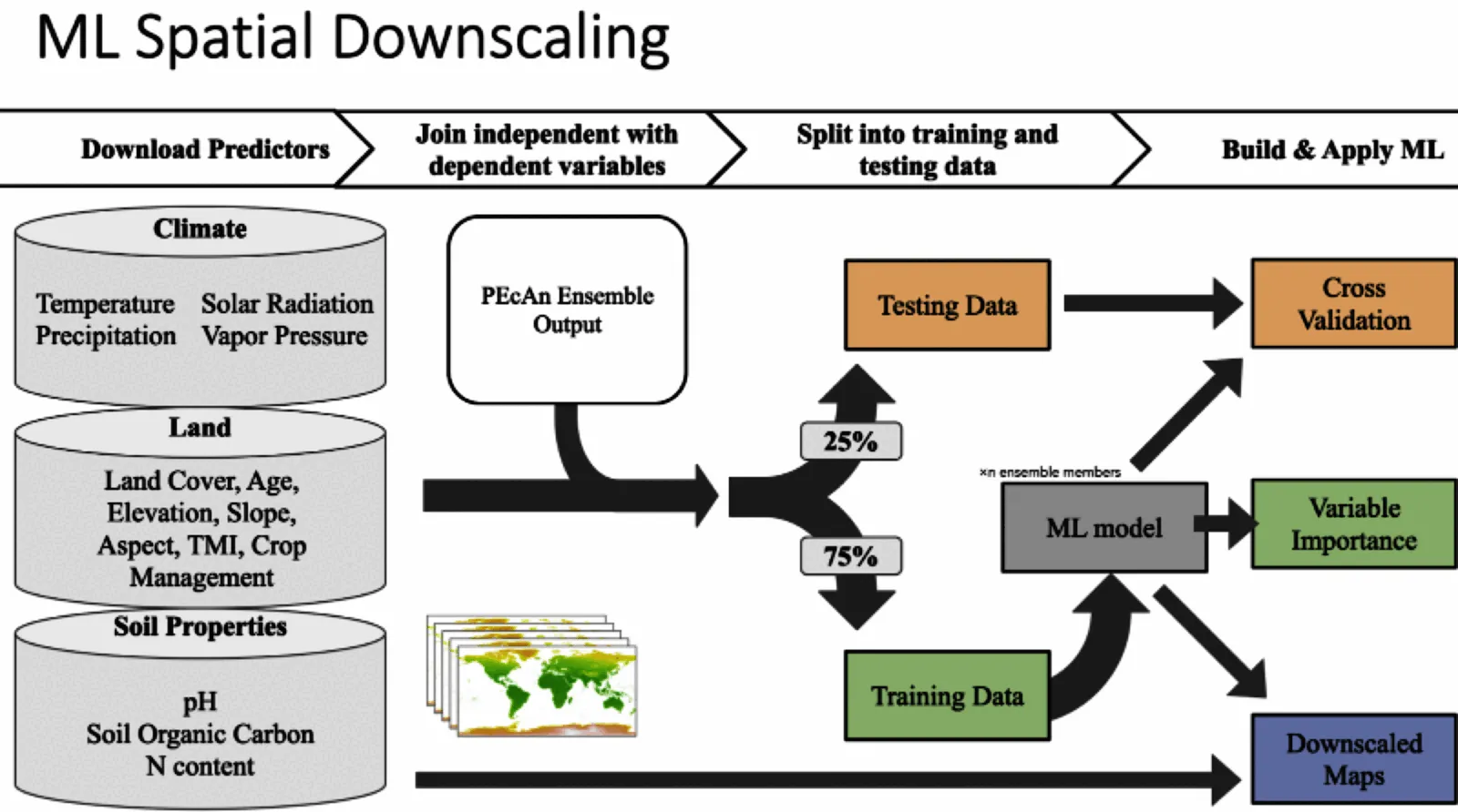
6. Downscale, Aggregate to County, and Plot

Rscript scripts/040_downscale.R
Rscript scripts/041_aggregate_to_county.R
Rscript scripts/042_downscale_analysis.R
Rscript scripts/043_county_level_plots.R

Builds Random Forest models to predict carbon pools for all fields; aggregates to county-level; summarizes variable importance; and produces maps:

• Train models on SIPNET ensemble runs at design points
• Use environmental covariates to downscale predictions to all fields
• Aggregate to county-level estimates
• Output maps and statistics of carbon density and totals

Inputs: - model_outdir/ensemble_output.csv: SIPNET outputs extracted in step 4 - data/site_covariates.csv: Environmental covariates

Outputs from 040_downscale.R: - model_outdir/downscaled_preds.csv: Per-site, per-ensemble predictions with columns: - site_id, scenario, pft, ensemble, c_density_Mg_ha, total_c_Mg, area_ha, county, model_output - model_outdir/downscaled_preds_metadata.json: Metadata including scenarios list - model_outdir/downscaled_deltas.csv: Carbon change from simulation start to end per scenario - model_outdir/training_sites.csv: Training site list per scenario, PFT, and pool - cache/models/*_models.rds: Saved RF models per spec - cache/training_data/*_training.csv: Training covariate matrices per spec

Outputs from 041_aggregate_to_county.R: - model_outdir/county_aggregated_preds.csv: County statistics per scenario with columns: - scenario, model_output, pft, county, n, mean_total_c_Tg, sd_total_c_Tg, mean_c_density_Mg_ha, sd_c_density_Mg_ha, mean_total_ha, sd_total_ha - model_outdir/county_aggregated_deltas.csv: County-level carbon change per scenario - model_outdir/state_summaries.csv: State-level totals per scenario - model_outdir/aggregation_metadata.json: Metadata for aggregated outputs

Outputs from 042_downscale_analysis.R (saved in figures/): - <pft>_<pool>_importance_partial_plots.png: Variable importance with partial plots for top predictors - <pft>_<pool>_ALE_predictor<i>.svg and <pft>_<pool>_ICE_predictor<i>.svg: ALE and ICE plots

Outputs from 043_county_level_plots.R (saved in figures/): - county_<scenario>_<pft>_<pool>_carbon_stock.webp: County-level stock maps per scenario - field_<scenario>_<pft>_<pool>_carbon_density.webp: Field-level density point maps per scenario - county_diff_woody_plus_annual_minus_woody_<pool>_carbon_stock.webp: Difference maps (mixed - woody) - stock only - county_delta_<scenario>_<pft>_<pool>_carbon_stock.webp: Start-to-end delta stock maps when available

Running on BU Cluster

Interactive session (example):

qrsh -l h_rt=3:00:00 -pe omp 16 -l buyin

Submit a batch job (example using downscaling step):

qsub \
  -l h_rt=4:00:00 \
  -pe omp 8 \
  -o logs/040.out \
  -e logs/040.err \
  -b y Rscript scripts/040_downscale.R

Documentation Site (Quarto)

• Preview: quarto preview
• Build: quarto render
• Publish to GitHub Pages: quarto publish gh-pages (publishes _site/)

Notes: - Quarto config is in _quarto.yml and the home page is index.qmd (includes README.md). - Uses freeze: auto to cache outputs; rebuild where data paths exist (see 000-config.R).

Technical Reference

Ensemble Structure

Each ensemble member represents a plausible realization given parameter and meteorological uncertainty. This ensemble structure is maintained throughout the workflow to properly propagate uncertainty. For example, downscaling is done for each ensemble member separately, and then the results are aggregated to county-level statistics.