Downscaling Results and Analysis

Overview

This page presents baseline results from the Random Forest downscaling of SIPNET model outputs from 100 anchor sites to approximately 132,000 annual cropland fields across 57 California counties. Results include county-level totals, field-level density maps, and mixed baseline-plus-scenario-difference comparisons for soil carbon, aboveground biomass, and GHG fluxes (N₂O, CH₄). For detailed interpretation of scenario effects, see the Soil Carbon Atlas and GHG Emissions Atlas.

Validation Status

These results are from a proof-of-concept modeling framework that has not been validated against field observations. Interpret all values as illustrative projections, not empirical estimates.

For detailed information about methods and workflow, see the Workflow Documentation.

County-Level Baseline Carbon Stocks

County-level maps show the total mass summed across all annual cropland fields in each county. Central Valley counties (Kern, Fresno, Tulare, San Joaquin) dominate because they contain the most cropland area. Units are Gg (gigagrams) for carbon pools and Gg yr⁻¹ for GHG fluxes.

Soil Carbon (TotSoilCarb)

County total soil carbon – Baseline. Statewide total: 112.3 Tg C at 30 cm depth.

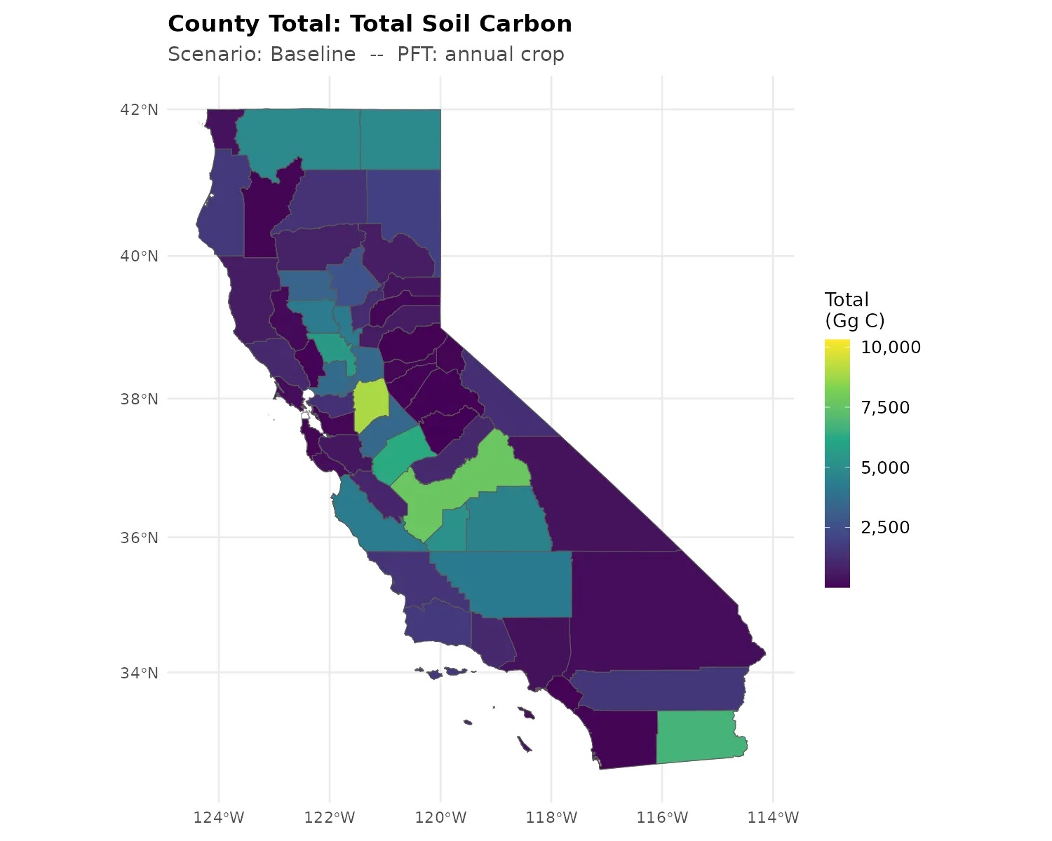
The spatial pattern reflects county-level cropland area more than per-hectare soil properties. Kern, Fresno, and Tulare counties show the highest totals because they contain the largest share of California’s annual cropland. See the field-level density maps below for the per-hectare view that isolates soil and climate effects from area.

Aboveground Biomass (AGB)

County total aboveground biomass – Baseline. Statewide total: approximately 40 Mg C.

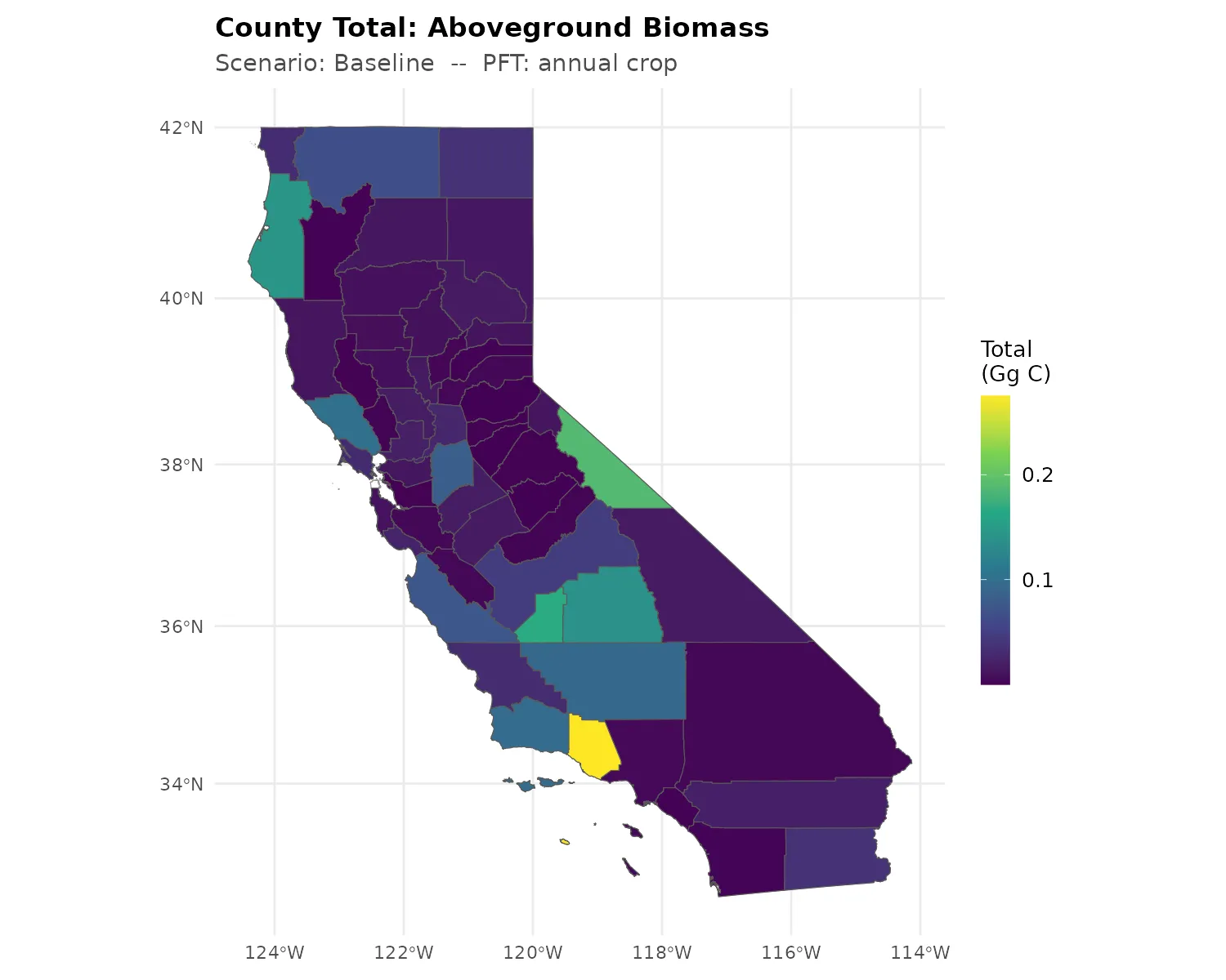
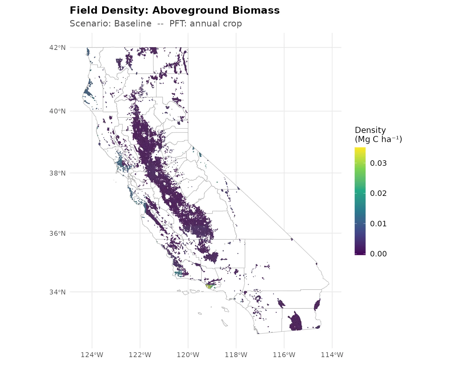
AGB in annual croplands reflects standing biomass at the modeled time point. Values are very small compared to soil carbon pools because annual crops are harvested. AGB is most useful as a relative indicator of crop productivity differences across regions.

Nitrous Oxide (N₂O) Flux

County total N₂O flux – Baseline. Statewide total: 12.91 Gg N₂O yr⁻¹.

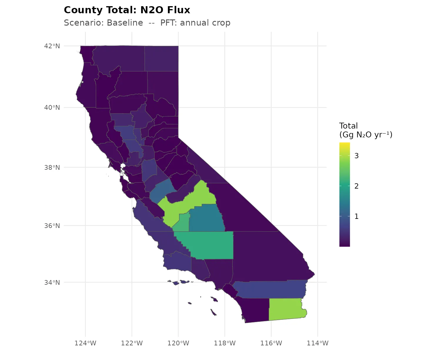
N₂O emissions are highest in the southern San Joaquin Valley (Kern, Tulare, Kings, Fresno) and Imperial County. This pattern reflects the combined influence of large cropland areas and warmer temperatures that promote nitrification and denitrification. The north-south gradient in per-hectare N₂O emission rates is driven by temperature and vapor pressure (see Model Drivers).

Methane (CH₄) Flux

County total CH₄ flux – Baseline. Statewide total: 0.014 Gg CH₄ yr⁻¹ – effectively zero.

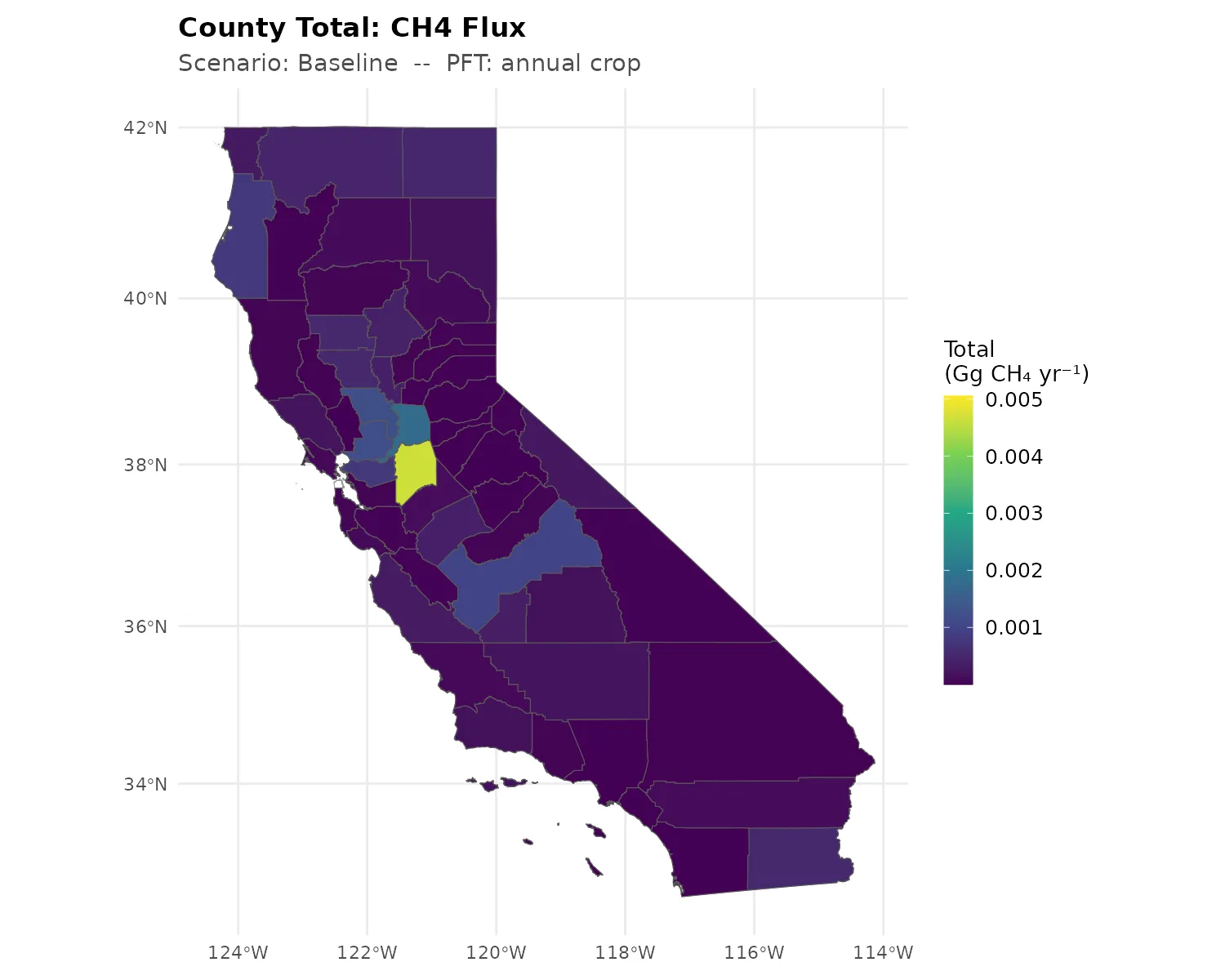
CH₄ Is Effectively Zero

Non-flooded annual croplands produce negligible CH₄ because methanogenesis requires sustained anaerobic conditions (continuous flooding) that do not occur under standard irrigation. The statewide total of 0.014 Gg CH₄ yr⁻¹ is effectively machine-precision zero in the process model. Any spatial pattern in this map reflects noise in the downscaling model (OOB R² = -0.15), not real ecological variation. Meaningful CH₄ fluxes are expected when rice paddies are included in future model runs.

Field-Level Baseline Density

Area-normalized density (per hectare) at the individual field level isolates per-area effects from county cropland area. These maps reveal how soil type, climate, and topography drive spatial variation independent of how much cropland each county contains.

Soil Carbon (TotSoilCarb)

Field-level soil carbon density – Baseline (Mg C ha⁻¹)

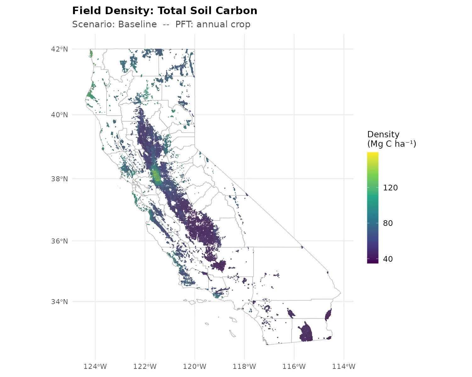
Sacramento Valley fields (north) tend to show higher per-hectare soil carbon than San Joaquin Valley fields (south), consistent with cooler temperatures slowing organic matter decomposition. This gradient is driven primarily by organic carbon density (ocd) and vapor pressure (vapr) – see Model Drivers.

Aboveground Biomass (AGB)

Field-level AGB density – Baseline (Mg C ha⁻¹)

Nitrous Oxide (N₂O) Flux

Field-level N₂O flux density – Baseline (kg N₂O ha⁻¹ yr⁻¹)

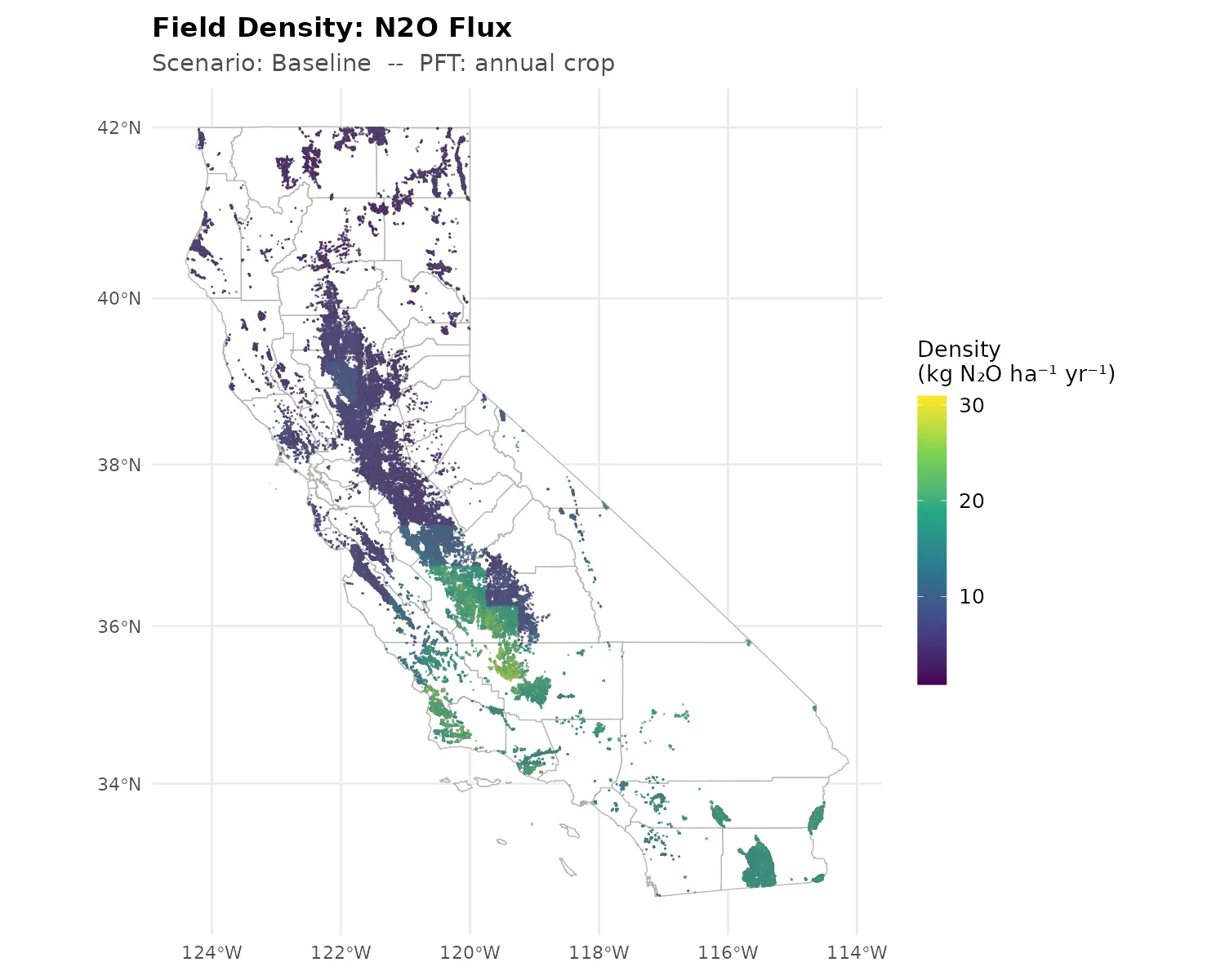
Per-hectare N₂O emissions show a clear north-south gradient: southern fields (Imperial Valley, southern San Joaquin) emit 20–30 kg N₂O ha⁻¹ yr⁻¹ while northern fields emit 5–10 kg N₂O ha⁻¹ yr⁻¹. This gradient reflects the strong temperature and vapor pressure dependence of soil N₂O production through nitrification and denitrification pathways.

Methane (CH₄) Flux

Field-level CH₄ flux density – Baseline (kg CH₄ ha⁻¹ yr⁻¹)

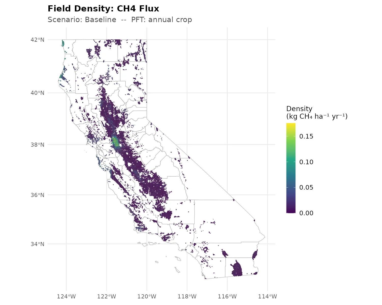
All field-level CH₄ values are effectively zero (0.007 kg CH₄ ha⁻¹ yr⁻¹ statewide average). Any spatial variation is noise from the downscaling model, not a real ecological signal.

Mixed Comparison: Baseline + Scenario Differences

These panels show the baseline map alongside the five scenario difference maps for each variable. The first panel uses an absolute scale; panels 2–6 use a diverging scale centered on zero. See the Scenario Definition Table for practice parameters and simulation details. For detailed interpretation, see the Soil Carbon Atlas and GHG Emissions Atlas.

Soil Carbon (TotSoilCarb)

Baseline absolute + scenario differences for total soil carbon

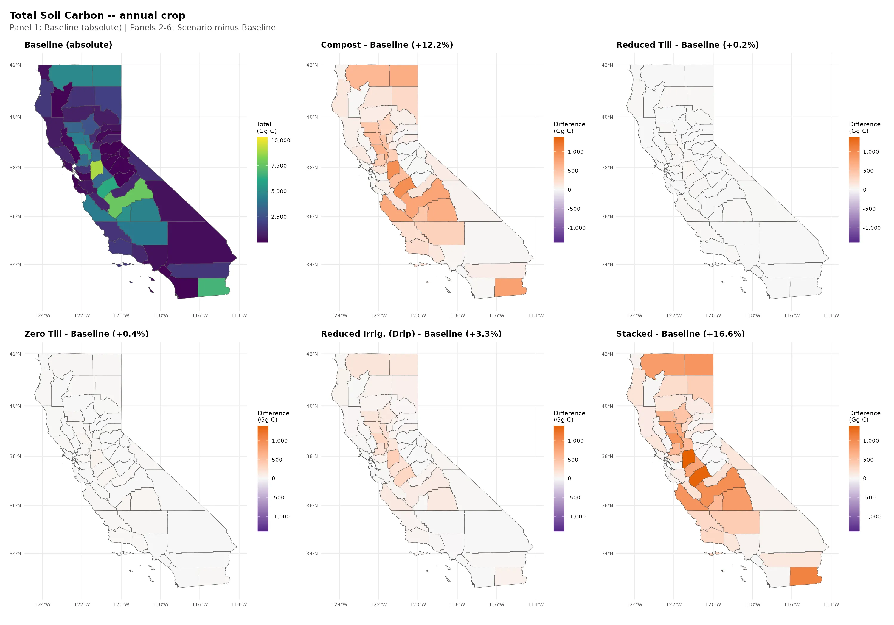
All five management scenarios increase soil carbon relative to baseline. Compost (+12.2%) and stacked (+16.6%) show the largest gains. See Soil Carbon Atlas for detailed scenario analysis.

Aboveground Biomass (AGB)

Baseline absolute + scenario differences for aboveground biomass

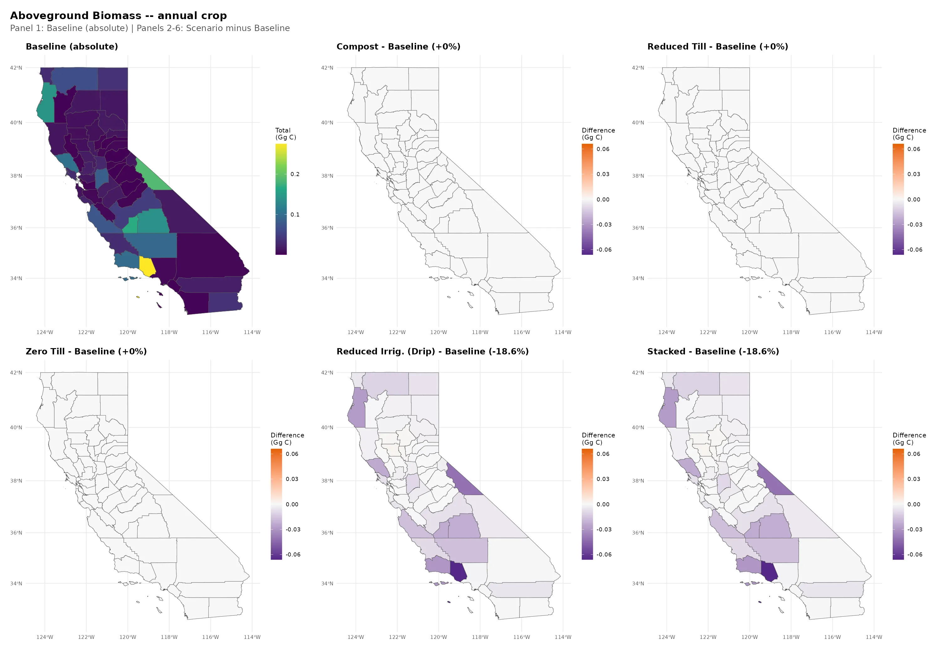
Compost and tillage scenarios show no AGB change (0%). Drip irrigation and stacked scenarios show -18.6% AGB reduction, reflecting altered water availability affecting end-of-season residue.

Nitrous Oxide (N₂O) Flux

Baseline absolute + scenario differences for N₂O flux

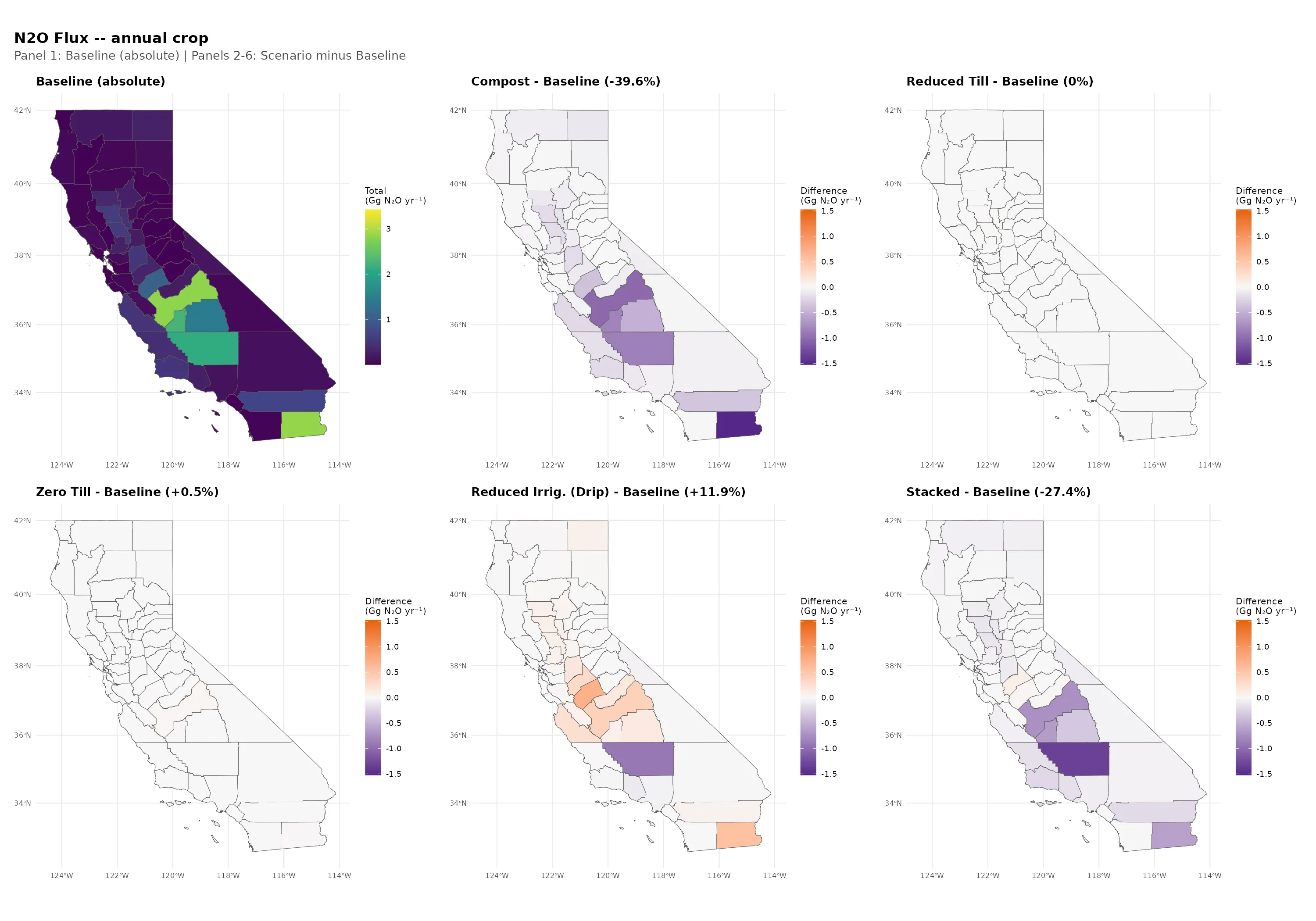
Compost (-39.5%) and stacked (-27.3%) reduce N₂O emissions. Drip irrigation (+12.0%) increases N₂O. Tillage scenarios show essentially no change. See GHG Emissions Atlas for detailed trade-off analysis.

Methane (CH₄) Flux

Baseline absolute + scenario differences for CH₄ flux

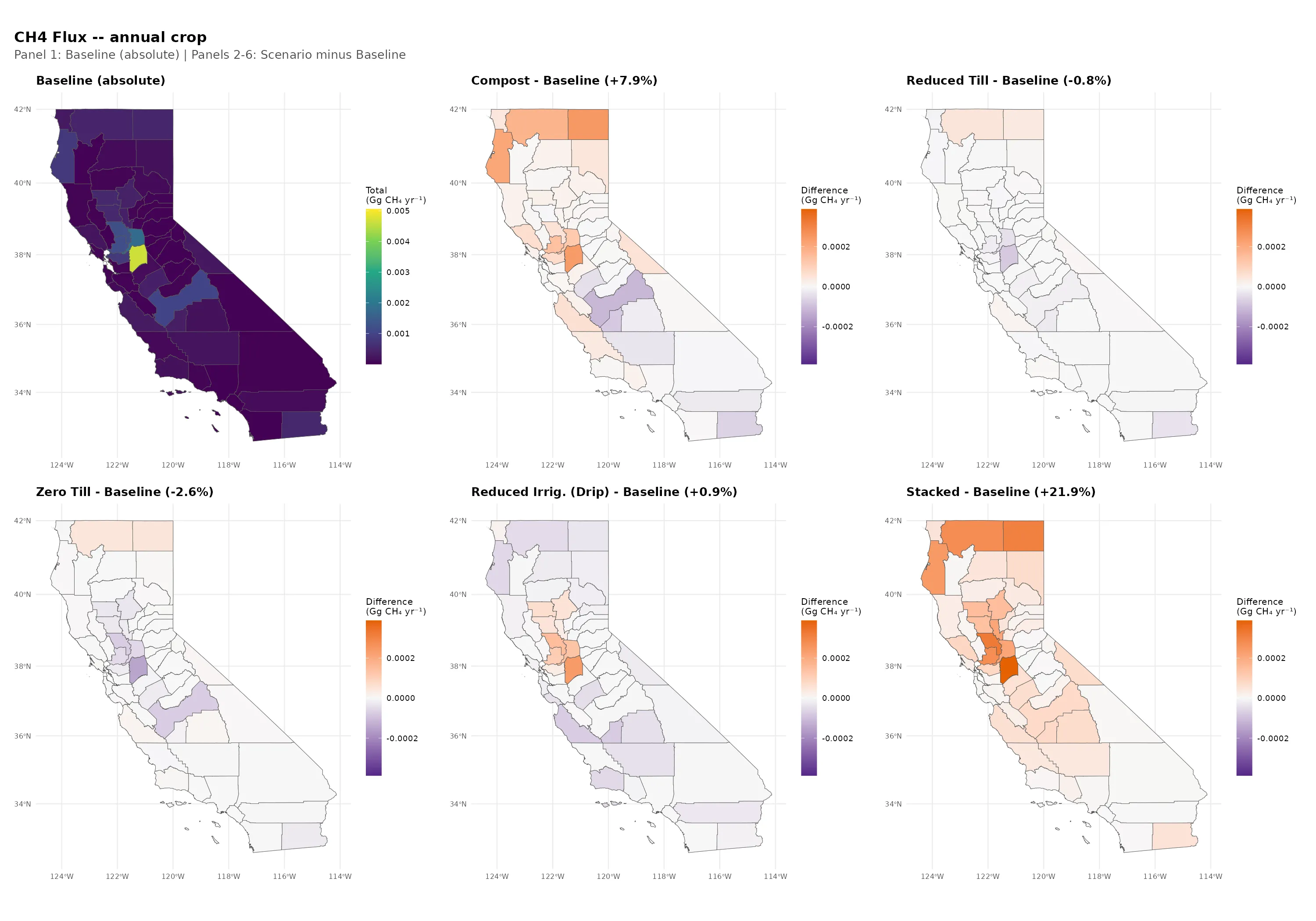
All CH₄ values are effectively zero for non-flooded annual croplands. Percentage differences shown in panel titles are misleading because the baseline is machine-precision zero. See the GHG Emissions Atlas for discussion.

Interactive Data Tables

County Stocks and Density (Baseline)