Downscaling Model Evaluation
Out-of-Bag Performance, Variable Importance, and Predictor Collinearity
This page summarizes model diagnostics for the Random Forest downscaling models used to predict SIPNET outputs from 100 anchor sites to approximately 132,000 annual cropland fields. For ecological interpretation of predictor effects (ALE/ICE plots), see the Model Drivers page.
These results are from a proof-of-concept modeling framework that has not been validated against field observations. Interpret all values as illustrative projections, not empirical estimates.
Out-of-Bag Performance
Out-of-bag (OOB) R² measures how well each Random Forest predicts held-out training sites. It is computed separately for each of 20 ensemble members; the table shows the median and interquartile range. OOB R² is a conservative estimate of spatial predictive accuracy because it uses only the approximately one-third of training sites not included in each bootstrap sample (each bootstrap draws n with replacement from n, leaving ~37% out-of-bag).
| Variable | Median OOB R² | IQR | Top 2 Predictors | Assessment |
|---|---|---|---|---|
| N2O Flux | 0.52 | 0.38–0.72 | vapr, temp | Best spatial model |
| TotSoilCarb | 0.34 | 0.26–0.41 | ocd, vapr | Moderate |
| AGB | 0.09 | -0.04–0.52 | precip, vapr | Poor – high variance across ensembles |
| CH4 Flux | -0.15 | -0.17 to -0.13 | none meaningful | No spatial signal (near-zero baseline) |
Non-flooded annual croplands produce negligible CH4 in SIPNET because methanogenesis requires sustained anaerobic conditions (continuous flooding) that do not occur under standard irrigation. The statewide baseline is approximately 14,000 kg CH4 yr⁻¹ – effectively zero. With no spatial variation in the training data, the Random Forest cannot distinguish signal from noise. The negative R² confirms the model performs worse than predicting the mean. CH4 importance rankings and ALE/ICE plots reflect noise, not ecology. Meaningful CH4 fluxes are expected when rice paddies are included in future model runs.
The AGB model’s wide IQR (-0.04 to 0.52) across ensembles means some ensemble members have no spatial predictive power while others are moderate. This inconsistency should be considered when interpreting AGB spatial maps. The low and variable R² likely reflects the fact that annual crop AGB at the modeled time point is small (post-harvest residue) and may not vary systematically with the environmental covariates used here.
Variable Importance
Variable importance is measured as the increase in mean squared error (MSE) when each predictor is randomly permuted while all others are held constant. Higher values indicate the model depends more on that variable for accurate predictions. Importance is summarized as the median across 20 ensemble members; error bars in the figure show the IQR.
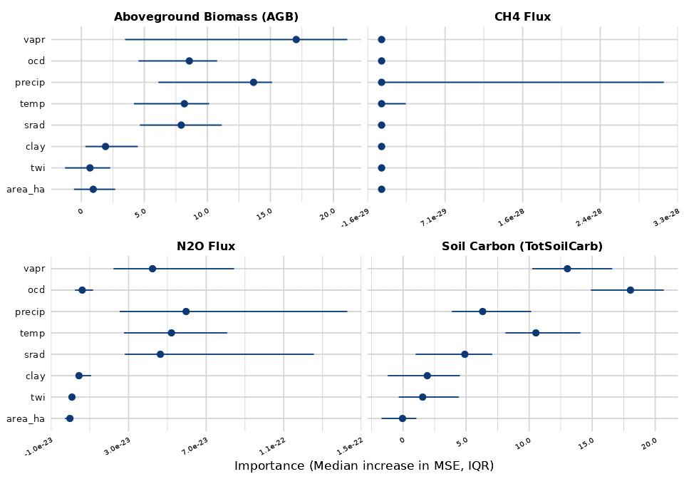
| Rank | TotSoilCarb | AGB | N2O Flux | CH4 Flux |
|---|---|---|---|---|
| 1 | ocd (18.4) | precip (9.7) | vapr | all near 0 |
| 2 | vapr (12.8) | vapr (8.7) | temp | all near 0 |
| 3 | temp (12.0) | ocd (7.9) | precip | all near 0 |
| 4 | precip (6.9) | temp (7.4) | srad | all near 0 |
Interpretation
Soil carbon is most strongly driven by existing organic carbon density (ocd), which is both a predictor and correlated with the output. This reflects the well-known positive feedback between soil organic matter and further C retention – SOM persistence is controlled by environmental and biological interactions rather than molecular recalcitrance alone (Schmidt et al. 2011, Nature). Climate variables (vapr, temp) rank second and third, capturing the temperature-driven decomposition gradient across California.
N2O flux is driven by climate variables (vapr, temp, precip), consistent with the well-established temperature and moisture sensitivity of soil nitrification and denitrification processes (Butterbach-Bahl et al. 2013, Philosophical Transactions of the Royal Society B). The dominance of vapor pressure likely reflects its strong correlation with temperature (r = 0.86); together they capture the north-south climate gradient that controls soil moisture availability for N-cycling microbes.
AGB shows precipitation and vapor pressure as top predictors, consistent with water availability limiting annual crop productivity in California’s Mediterranean climate. However, the low and variable R² means these relationships are not reliably captured.
CH4 flux shows no meaningful importance for any predictor, confirming the training data contains no spatial signal for the model to learn.
Predictor Collinearity
The environmental predictors are correlated due to California’s climate gradients. High collinearity does not bias Random Forest predictions, but it does affect the interpretability of individual predictor importance: when two predictors are correlated, their importance is split between them, and their individual rankings become unstable. This is why we use ALE plots (which handle correlated predictors correctly) rather than Partial Dependence Plots for ecological interpretation.
| Predictor Pair | Pearson r | Severity |
|---|---|---|
| temp – vapr | +0.86 | Strong |
| precip – srad | -0.86 | Strong |
| srad – vapr | +0.58 | Moderate |
| temp – precip | -0.56 | Moderate |
| ocd – vapr | -0.55 | Moderate |
| temp – srad | +0.54 | Moderate |
| precip – vapr | -0.52 | Moderate |
| ocd – srad | -0.53 | Moderate |
| ocd – precip | +0.49 | Moderate |
The two strongest correlations – temp/vapr and precip/srad – reflect California’s dominant climate gradients:
- Temperature and vapor pressure (r = 0.86): Both increase from north to south along the Central Valley. This means the downscaling model cannot fully distinguish whether soil carbon losses or N2O increases in warmer areas are driven by temperature per se or by the correlated increase in atmospheric moisture demand.
- Precipitation and solar radiation (r = -0.86): Wetter areas (north coast, Sierra foothills) receive less direct solar radiation. This inverse relationship reflects the basic climate physics of cloud cover and California’s coastal-inland gradient.
These collinearities are an inherent feature of California’s climate geography, not a modeling artifact. They should be kept in mind when interpreting individual predictor effects in the Model Drivers plots.