Intro to MAGiC Downscaling

Overview

This document gives a brief overview of the MAGiC downscaling pipeline. The downscaling workflow follows the ensemble workflow: it starts from SIPNET NetCDF outputs from a subset of representative design points, uses machine learning to downscale to field-level carbon predictions, and then aggregates to county-level statistics.

flowchart LR
    A["PEcAn/SIPNET NetCDF outputs"] --> B["Extract to CSV<br/>script 030"]
    B --> C["Downscale to fields<br/>script 040"]
    C --> D["Aggregate to county<br/>script 041"]

For this intro we focus on soil carbon (TotSoilCarb) for one ensemble member of the baseline scenario in 2024. Other model outputs, including but not limited to aboveground biomass and GHG fluxes (N2O, CH4), can be downscaled and aggregated with the same pipeline.

Pre-requisites for this demo include:

• System setup
  • AWS CLI
  • A Conda environment
  • The github.com/ccmmf/downscaling repository cloned locally
  • A Linux computing environment
• Input data – two archives downloaded from S3 storage:
  • Output from SIPNET runs at design points
  • CADWR Land Use Maps

This tutorial will cover the following components:

1. Workflow Overview: how SIPNET outputs become field-level predictions and county-level aggregates
2. Extract SIPNET output: script 030 converts NetCDF files to ensemble_output.csv
3. Downscale to fields: script 040 fits Random Forest models and predicts to fields
4. Inspect outputs: look at tables and quick plots to understand the downscaled predictions
5. Wrap-up: recap and aggregation preview

Demo Mode This demo runs a simplified version of the pipeline to focus on the core downscaling steps. The full pipeline includes more variables, scenarios, and ensemble members, which add complexity but follow the same overall structure.

The --mode demo flags in the commands below constrain the pipeline to a single slice of the data:

• One variable (TotSoilCarb) is downscaled
• One scenario (baseline), so it does not include scenario-vs-baseline comparisons.
• One ensemble member

Demo mode does not include scenario-vs-baseline comparisons or ensemble based uncertainty analysis.

Outputs:

Demo mode does not include scenario-vs-baseline comparisons or ensemble based uncertainty analysis.

Outputs: * ensemble_output.csv – monthly SIPNET output in long format * downscaled_preds.csv – per-field carbon predictions

System setup

The pipeline runs inside a conda environment that includes the software required by the downscaling scripts.

The demo data and the pecan-all env tarball are downloaded from an S3 bucket hosted at NCSA.

If you have already set up your Conda environment, run the following. Otherwise, proceed with the setup steps below.

conda activate ~/.conda/envs/pecan-all
## Check AWS access

First, confirm that the AWS CLI is available:

```bash
aws --version

If that command is not found, load the AWS CLI as a module on your HPC system or install it from the AWS CLI installation instructions.

Next, confirm that you can read the CCMMF S3 bucket:

aws s3 ls s3://carb/data_raw/

If the bucket listing fails because of missing credentials, configure the ccmmf-garage profile.

Add this section to ~/.aws/credentials:

[ccmmf-garage]
aws_access_key_id = [your key ID]
aws_secret_access_key = [your secret key]

Add this section to ~/.aws/config:

[profile ccmmf-garage]
region = garage
endpoint_url = https://s3.garage.ccmmf.ncsa.cloud

Make sure the credential files are readable only by you:

chmod 600 ~/.aws/credentials ~/.aws/config

Activate the profile for the current shell and check access again:

export AWS_PROFILE=ccmmf-garage
aws s3 ls s3://carb/data_raw/

Setup Conda environment

We will use a conda environment that provides R, PEcAn, and all of the R packages the pipeline scripts depend on. The environment is available as a tarball on S3.

In this example, ~/.conda/envs/pecan-all is the target location, but you may want to put this somewhere other than your home directory.

Note that this may take 30 minutes or more to download and install.

aws s3 cp s3://carb/deploy/setup-pecan-env.sh ./
bash setup-pecan-env.sh 1.10 ~/.conda/envs/pecan-all

To activate the pecan-all environment in a new shell:

conda activate ~/.conda/envs/pecan-all

Clone the downscaling repository

The pipeline scripts live in the downscaling repo, which is located at https://github.com/ccmmf/downscaling. Clone the repository to your working directory – the rest of the steps below assume you’re inside the cloned directory.

git clone -b develop https://github.com/ccmmf/downscaling.git
cd downscaling

Input data

We install two data archives from S3. The first is the demo subset of SIPNET outputs (baseline scenario, ensemble 1, year 2024). The second is a vector file of California crop fields and county geometry layers derived from the CADWR Land Use Dataset [Cite].

mkdir -p ~/ccmmf_demo/modelout ~/ccmmf_demo/data

aws s3 cp s3://carb/data_raw/ccmmf_phase_3_scenarios_v2_n2o_ch4_demo.tgz - | \
  tar xzf - -C ~/ccmmf_demo/modelout/

aws s3 cp s3://carb/data_raw/ccmmf_downscaling_data_layers.tgz - | \
  tar xzf - -C ~/ccmmf_demo/data/

Note: to run a full production run, you can download ccmmf_phase_3_scenarios_v2_n2o_ch4.tgz. This is about 95 GB and may take 30 minutes or longer to download.

Verify the layout:

ls ~/ccmmf_demo/modelout/ccmmf_phase_3_scenarios_v2_n2o_ch4/
ls ~/ccmmf_demo/data/

In modelout/... you should see output_baseline/ and site_info.csv. In data/ you should see ca_fields.gpkg, ca_field_attributes.csv, site_covariates.csv, and ca_counties.gpkg.

These are the PEcAn model output files that script 030 will extract:

find ~/ccmmf_demo/modelout/ccmmf_phase_3_scenarios_v2_n2o_ch4/output_baseline/out \
  -name "2024.nc" | head

What does one of these files contain?

ncdump -h $(find ~/ccmmf_demo/modelout/ccmmf_phase_3_scenarios_v2_n2o_ch4/output_baseline/out \
  -name "2024.nc" | head -n1)

Show the covariate table that script 040 will use:

head -n 5 ~/ccmmf_demo/data/site_covariates.csv | column -s, -t

Set the CCMMF_DIR environment variable so that the pipeline knows where to find the data:

export CCMMF_DIR=~/ccmmf_demo

This tells the pipeline where to find $CCMMF_DIR/modelout/... and $CCMMF_DIR/data/..., as well as where to write pipeline outputs.

Extract SIPNET output

The 030_extract_sipnet_output.R script reads the PEcAn standard netCDF model output, aggregates to monthly values, and writes these values to a long CSV, ensemble_output.csv.

Let’s run it in demo mode:

Rscript scripts/030_extract_sipnet_output.R --mode demo

Confirm and inspect the output:

ls -lh ~/ccmmf_demo/modelout/ccmmf_phase_3_scenarios_v2_n2o_ch4/ensemble_output.csv
head -n 5 ~/ccmmf_demo/modelout/ccmmf_phase_3_scenarios_v2_n2o_ch4/ensemble_output.csv | column -s, -t

ensemble_output <- readr::read_csv(file.path(model_outdir, "ensemble_output.csv"),
  show_col_types = FALSE)
dplyr::glimpse(ensemble_output)

Rows: 1,200
Columns: 10
$ scenario      <chr> "baseline", "baseline", "baseline", "baseline", "baselin…
$ datetime      <dttm> 2024-01-01, 2024-02-01, 2024-03-01, 2024-04-01, 2024-05…
$ site_id       <chr> "02f8ecd6d492badc", "02f8ecd6d492badc", "02f8ecd6d492bad…
$ lat           <dbl> 36.30494, 36.30494, 36.30494, 36.30494, 36.30494, 36.304…
$ lon           <dbl> -121.1654, -121.1654, -121.1654, -121.1654, -121.1654, -…
$ pft           <chr> "annual crop", "annual crop", "annual crop", "annual cro…
$ parameter     <dbl> 1, 1, 1, 1, 1, 1, 1, 1, 1, 1, 1, 1, 1, 1, 1, 1, 1, 1, 1,…
$ variable      <chr> "TotSoilCarb", "TotSoilCarb", "TotSoilCarb", "TotSoilCar…
$ variable_type <chr> "pool", "pool", "pool", "pool", "pool", "pool", "pool", …
$ prediction    <dbl> 4.299215, 4.298731, 4.298046, 4.296897, 4.293167, 4.2837…

ensemble_output |>
  dplyr::summarise(
    rows = dplyr::n(),
    sites = dplyr::n_distinct(site_id),
    ensembles = dplyr::n_distinct(parameter),
    variables = paste(unique(variable), collapse = ", "),
    start = min(datetime),
    end = max(datetime)
  )

# A tibble: 1 × 6
   rows sites ensembles variables   start               end                
  <int> <int>     <int> <chr>       <dttm>              <dttm>             
1  1200   100         1 TotSoilCarb 2024-01-01 00:00:00 2024-12-01 00:00:00

Downscaling from Model Outputs to fields

Now that we have extracted the model outputs to a tabular format, we can use these outputs to train machine learning models that predict field-level carbon stocks and fluxes.

This happens in scripts/040_downscale.R.

For each run, scripts/040_downscale.R:

1. Loads ensemble_output.csv, site covariates, and field attributes.
2. Iterates over each (scenario, PFT, carbon pool) combination.
3. Fits one Random Forest model per ensemble member for that combination.
4. Predicts field level density for that PFT, output column density_per_ha (Mg C / ha for stocks, kg/ha/yr for fluxes).
5. Multiplies density by each field’s area to derive total stock per field: total_per_field = density_per_ha * area_ha.
6. Writes outputs including downscaled_preds.csv (and .parquet for large outputs), with columns: site_id, scenario, pft, ensemble, density_per_ha, total_per_field, area_ha, county, model_output.

Fitting one RF model per ensemble member preserves and propagates uncertainty structure throughout the full modeling workflow.

Rscript scripts/040_downscale.R --mode demo

In demo mode there is one (scenario, PFT, pool) combo and one ensemble member and it predicts to roughly 10,000 target fields within a couple of minutes.

Outputs are written to $CCMMF_DIR/modelout/.../downscaled_preds.csv (and .parquet).

Inspect downscaled outputs

ls -lh ~/ccmmf_demo/modelout/ccmmf_phase_3_scenarios_v2_n2o_ch4/downscaled_preds.csv

model_outdir <- "~/ccmmf_demo/modelout/ccmmf_phase_3_scenarios_v2_n2o_ch4"
preds <- readr::read_csv(file.path(model_outdir, "downscaled_preds.csv"), show_col_types = FALSE)
dplyr::glimpse(preds)
preds |>
  dplyr::summarise(
    rows = dplyr::n(),
    fields = dplyr::n_distinct(site_id),
    counties = dplyr::n_distinct(county),
    min_density = min(density_per_ha, na.rm = TRUE),
    mean_density = mean(density_per_ha, na.rm = TRUE),
    max_density = max(density_per_ha, na.rm = TRUE)
  )

Focus on density_per_ha, scenario, pft, ensemble, county, and model_output. The area_ha column is useful later for converting density to total field carbon, but it is not the main explanatory variable for this first demo.

Make quick plots

Use density_per_ha for the first plot because it is the direct field-level downscaling result.

library(dplyr)
library(ggplot2)
library(readr)

preds <- read_csv(file.path(model_outdir, "downscaled_preds.csv"), show_col_types = FALSE)

ggplot(preds, aes(x = density_per_ha)) +
  geom_histogram(bins = 40, fill = "steelblue", color = "white") +
  labs(
    title = "Downscaled Total Soil Carbon",
    x = "Density (Mg C / ha)",
    y = "Number of fields"
  ) +
  theme_minimal()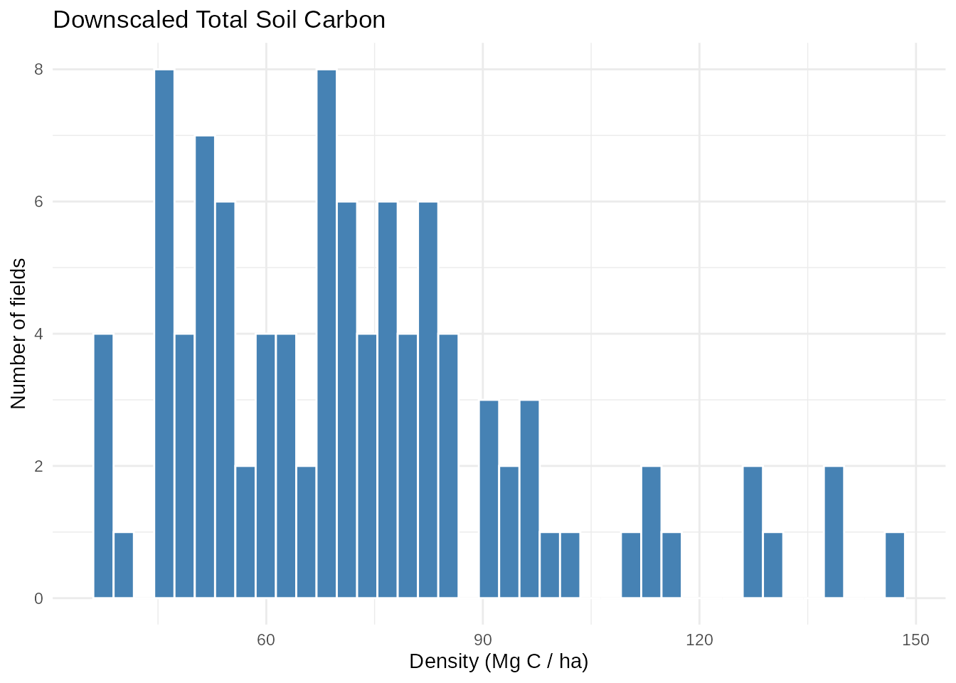

Join predictions to covariates to show how predicted soil carbon varies with a predictor such as organic carbon density (ocd) or temperature (temp).

covariates <- read_csv(file.path(data_dir, "site_covariates.csv"), show_col_types = FALSE)

plot_data <- preds |>
  left_join(
    covariates |> select(site_id, ocd, temp, vapr, clay, precip, srad, twi),
    by = "site_id"
  ) |>
  filter(!is.na(ocd), !is.na(density_per_ha))

plot_sample <- plot_data |>
  slice_sample(n = min(nrow(plot_data), 5000))

ggplot(plot_sample, aes(x = ocd, y = density_per_ha)) +
  geom_point(alpha = 0.25, size = 0.7) +
  geom_smooth(method = "loess", formula = y ~ x, se = FALSE, color = "black") +
  labs(
    title = "Predicted Soil Carbon vs. Soil Organic Carbon Density",
    x = "SoilGrids organic carbon density covariate",
    y = "Predicted density (Mg C / ha)"
  ) +
  theme_minimal()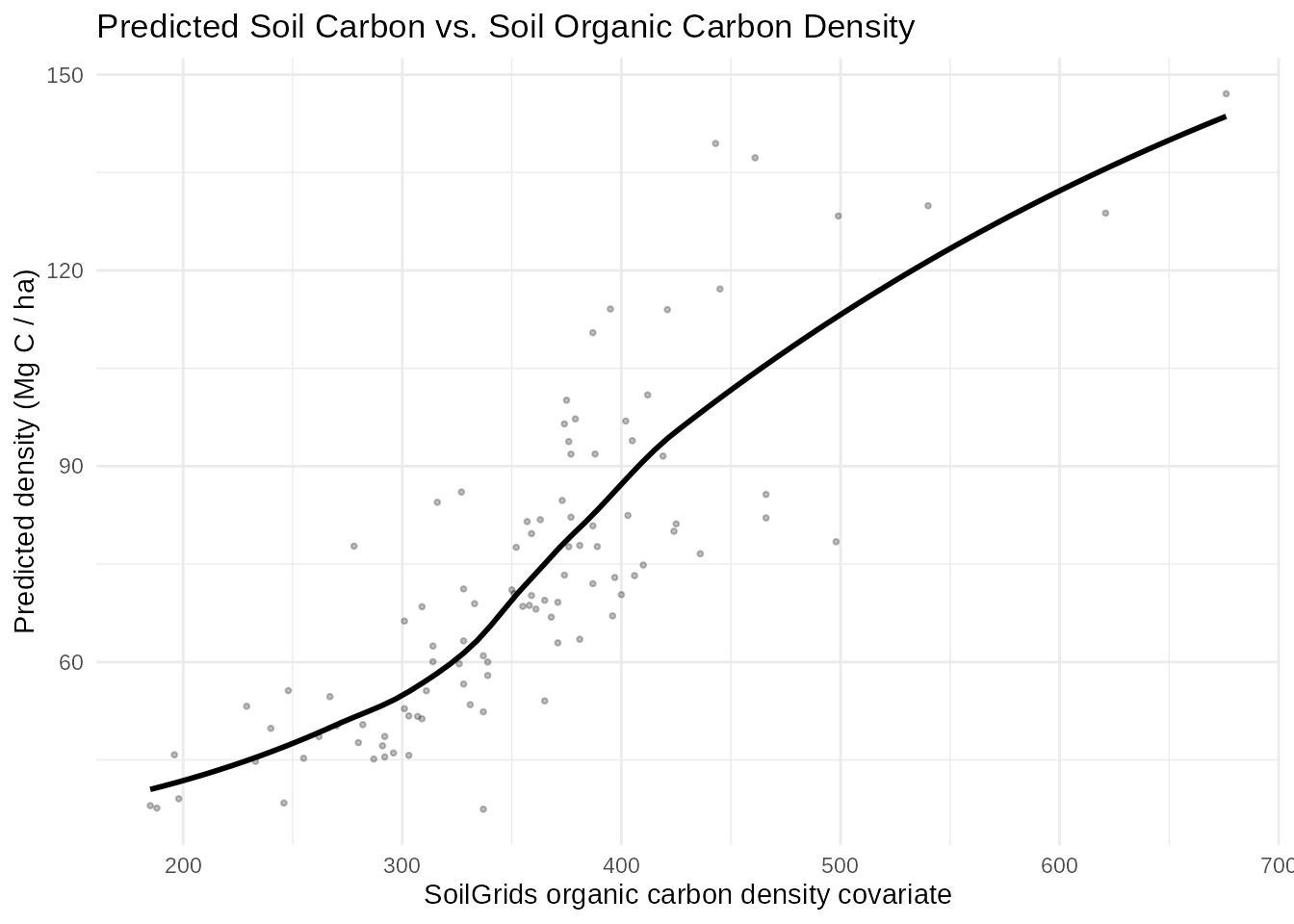

Aggregate to county

In previous steps, the downscaling pipeline produced field-level estimates of soil carbon density and total soil carbon. For reporting, mapping, and scenario comparison, we aggregate these to regional statistics.

Here we demonstrate how to summarize county level total soil carbon stocks.

Aggregation is performed by the scripts/041_aggregate_to_county.R script. That script reads downscaled_preds.csv that was generated in the previous step. This file contains the total stocks or fluxes (total soil carbon in this example) and the county name for each field.

It then groups field predictions by scenario, model output, county, and ensemble member, and then computes county level statistics.

To run the aggregation step in demo mode:

Rscript scripts/041_aggregate_to_county.R --mode demo

In demo mode, this step uses a small sample of fields per county. That keeps the demonstration fast, but the resulting county totals aren’t intended as the realistic estimates that are produced by a production run.

Output from the aggregation steps include:

• county_aggregated_preds.csv – county summaries by scenario, output variable, PFT, and county
• state_summaries.csv – statewide totals summarized across counties
• aggregation_metadata.json – a small description of the aggregation run and output columns
• county_aggregated_deltas.csv – county scenario deltas, when downscaled_deltas.csv exists

Because this first demo only includes the baseline scenario, there are no scenario-vs-baseline deltas to aggregate as there are in the development and production runs.

Confirm that the main aggregation outputs were created:

ls -lh ~/ccmmf_demo/modelout/ccmmf_phase_3_scenarios_v2_n2o_ch4/county_aggregated_preds.csv
ls -lh ~/ccmmf_demo/modelout/ccmmf_phase_3_scenarios_v2_n2o_ch4/state_summaries.csv

Inspect the county output:

head -n 5 ~/ccmmf_demo/modelout/ccmmf_phase_3_scenarios_v2_n2o_ch4/county_aggregated_preds.csv | column -s, -t

county_preds <- readr::read_csv(
  file.path(model_outdir, "county_aggregated_preds.csv"),
  show_col_types = FALSE
)

dplyr::glimpse(county_preds)

Rows: 35
Columns: 11
$ scenario              <chr> "baseline", "baseline", "baseline", "baseline", …
$ model_output          <chr> "TotSoilCarb", "TotSoilCarb", "TotSoilCarb", "To…
$ pft                   <chr> "annual crop", "annual crop", "annual crop", "an…
$ county                <chr> "Butte", "Calaveras", "Colusa", "Contra Costa", …
$ n                     <dbl> 2, 2, 2, 2, 5, 1, 2, 8, 4, 1, 2, 7, 1, 8, 2, 2, …
$ mean_total_per_county <dbl> 2410.0, 432.0, 5390.0, 1150.0, 445.0, 1800.0, 26…
$ sd_total_per_county   <lgl> NA, NA, NA, NA, NA, NA, NA, NA, NA, NA, NA, NA, …
$ mean_density_per_ha   <dbl> 74.4, 95.0, 65.0, 116.0, 51.3, 63.2, 129.0, 47.7…
$ sd_density_per_ha     <lgl> NA, NA, NA, NA, NA, NA, NA, NA, NA, NA, NA, NA, …
$ mean_total_ha         <dbl> 32.356564, 4.551630, 82.943513, 9.907703, 8.6790…
$ sd_total_ha           <lgl> NA, NA, NA, NA, NA, NA, NA, NA, NA, NA, NA, NA, …

county_preds |>
  dplyr::summarise(
    rows = dplyr::n(),
    counties = dplyr::n_distinct(county),
    scenarios = paste(unique(scenario), collapse = ", "),
    variables = paste(unique(model_output), collapse = ", "),
    pfts = paste(unique(pft), collapse = ", "),
    min_total = min(mean_total_per_county, na.rm = TRUE),
    mean_total = mean(mean_total_per_county, na.rm = TRUE),
    max_total = max(mean_total_per_county, na.rm = TRUE)
  )

# A tibble: 1 × 8
   rows counties scenarios variables   pfts       min_total mean_total max_total
  <int>    <int> <chr>     <chr>       <chr>          <dbl>      <dbl>     <dbl>
1    35       35 baseline  TotSoilCarb annual cr…      66.4      2888.     12800

Key columns in county_preds are:

• mean_total_per_county – mean county total across ensemble members
• sd_total_per_county – across-ensemble standard deviation of county totals
• mean_density_per_ha – area-weighted county density
• mean_total_ha – summed field area represented in the aggregation
• n – number of field predictions used in that county group

In this demo there is only one ensemble member, so there is no standard deviation.

Plot the largest county totals in the demo output:

top_counties <- county_preds |>
  dplyr::filter(model_output == "TotSoilCarb") |>
  dplyr::slice_max(mean_total_per_county, n = 15) |>
  dplyr::mutate(county = stats::reorder(county, mean_total_per_county))

ggplot2::ggplot(top_counties, ggplot2::aes(x = mean_total_per_county, y = county)) +
  ggplot2::geom_col(fill = "steelblue") +
  ggplot2::labs(
    title = "Largest County Soil Carbon Totals in the Demo Aggregation",
    x = "Mean county total (Mg C)",
    y = NULL
  ) +
  ggplot2::theme_minimal()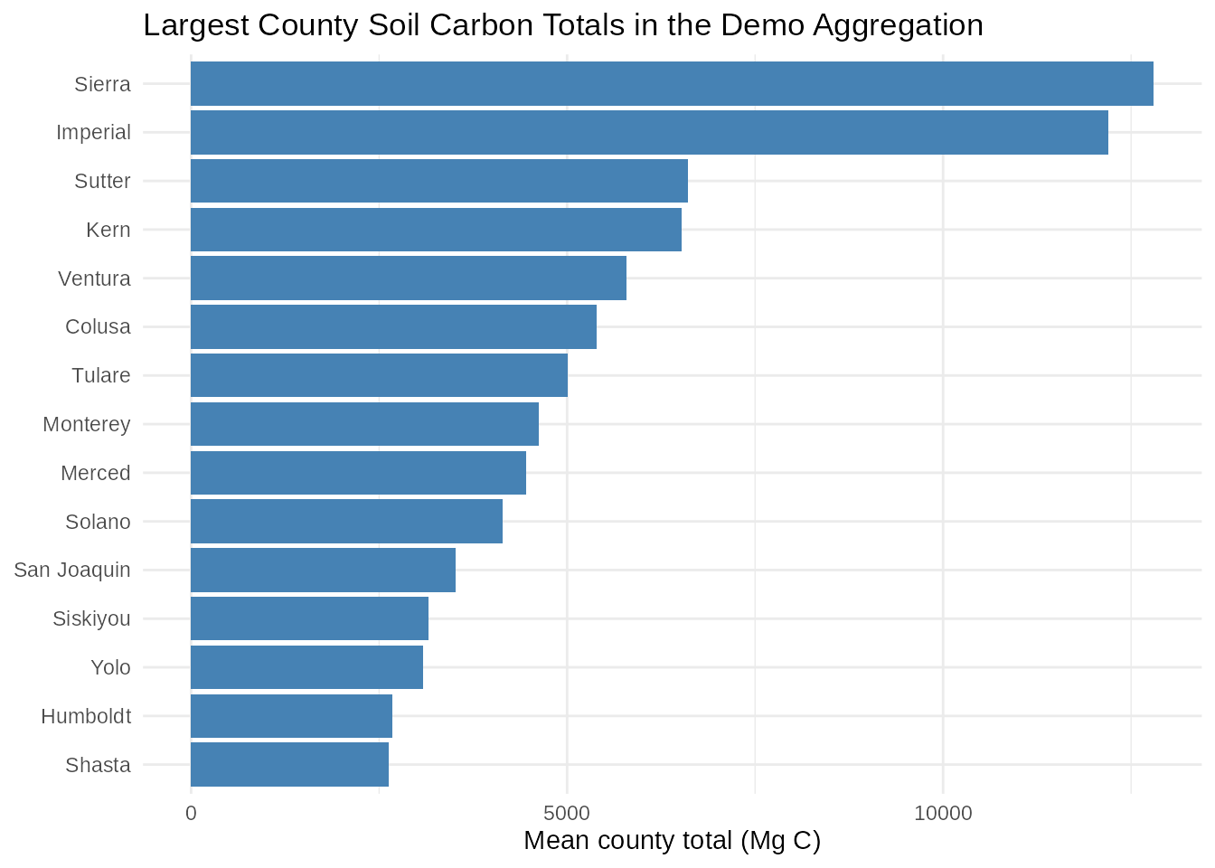

At this point, the pipeline has moved from model outputs at representative design points, to field-level predictions, to county and state summaries. The remaining follow-up scripts use these tables to make diagnostic plots and maps.

Next steps

• Other variables: AGB, N2O flux, CH4 flux. Same pipeline, different reporting units – Mg/ha for stocks, kg/ha/yr for fluxes.
• Development mode: use --mode dev and run with ensembles and at a larger range of sites and variables, but still in a computationally efficient manner.
  • Look at outputs for N2O and CH4 fluxes, and CO2e to compare across different components of crop GHG balance.